Summary

🎯 Voice Activity Detection (VAD), or voice endpoint detection, identifies time segments in an audio signal containing speech. This is a critical preprocessing step for automatic speech recognition (ASR) and voice wake-up systems. This project lays the groundwork for my upcoming ASR project 🤭.

📈 Workflow Overview: The VAD pipeline processes a speech signal as follows:

Preprocessing: Apply pre-emphasis to enhance high-frequency components.
Framing: Segment the signal into overlapping frames with frame-level labels.
Windowing: Apply window functions to mitigate boundary effects.
Feature Extraction: Extract a comprehensive set of features (e.g., short-time energy, zero-crossing rate, MFCCs, and more).
Binary Classification: Train models (DNN, Logistic Regression, Linear SVM, GMM) to classify frames as speech or non-speech.
Time-Domain Restoration: Convert frame-level predictions to time-domain speech segments.

🍻 Project Highlights: I conducted extensive experiments comparing frame division methods (frame length and shift) and model performances, with rich visualizations. For details, see the report in vad/latex/. If you’re interested in voice technologies, let’s connect!

For Chinese report, please see this article.

Methodology

1. Preprocessing

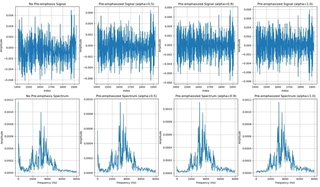
Pre-emphasis enhances high-frequency components to reduce spectral leakage.

$$ y[n] = x[n] - \alpha x[n-1] $$

where $x[n]$ is the input signal, $y[n]$ is the output, and $\alpha$ (typically 0.95–0.97) controls emphasis strength.

Pre-emphasis Impact:
Effect of pre-emphasis with varying $\alpha$

2. Framing

The signal is divided into overlapping frames. For signal length $N$, frame length $L$, and frame shift $S$, the number of frames $n_{\text{frames}}$ is:

Without zero-padding (floor):
$$ n_{\text{frames}} = \left\lfloor \frac{N - L}{S} \right\rfloor + 1 $$
With zero-padding (ceiling):
$$ n_{\text{frames}} = \left\lceil \frac{N - L}{S} \right\rceil + 1 $$
Zero-padding length:
$$ n_{\text{paddle}} = (n_{\text{frames}} - 1) \cdot S + L - N $$

3. Windowing

A window function (e.g., Hamming) is applied to each frame.

$$ x_i^{\text{windowed}}[n] = x_i[n] \cdot w[n], \quad 0 \leq n < L $$

Window Type Comparison:
Impact of window functions (e.g., Hamming, Hanning)

4. Feature Extraction

Extracted features (total dimension: 69) include:

Short-Time Energy (dimension: 1):
Measures frame energy, indicating loudness:
$$ E = \sum_{i=0}^{L-1} s_i^2 $$
where $s_i$ is the $i$-th sample in the frame, and $L$ is the frame length.
Frame-level energy plots:
Short-Time Zero-Crossing Rate (dimension: 1):
Counts zero crossings to distinguish voiced/unvoiced speech:
$$ Z = \frac{1}{2} \sum_{i=0}^{L-1} \left| \text{sgn}(s_i) - \text{sgn}(s_{i-1}) \right|, \quad \text{sgn}(x) = \begin{cases} 1, & x \geq 0 \\ 0, & x < 0 \end{cases} $$
Visualizing zero-crossing patterns:
Fundamental Frequency (Pitch) (dimension: 1):
Estimated via autocorrelation, representing the fundamental frequency:
$$ R(\tau) = \sum_{n=0}^{L-1-\tau} s[n] s[n+\tau], \quad f_0 = \frac{f_s}{\tau_{\text{max}}} $$
where $R(\tau)$ is the autocorrelation, $\tau_{\text{max}}$ is the lag maximizing $R(\tau)$, $f_s$ is the sampling frequency (16 kHz), and $s[n]$ is the frame signal.
And I have tried many smooth methods, see it in my report.
Spectral Mean (dimension: 1):
Indicates the spectral “center of mass”
$$ \mu_n = \frac{\sum_{k=1}^K\mid X(n, k)\mid}{K} $$
where $X(n, k)$ is the Fourier transform magnitude at bin $k$ in $n-$th frame, and $K$ is the number of bins.
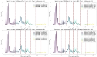
Sub-band Energies (dimension: 6):
$$ E_m = \sum_{k \in B_m} |S(k)|^2, \quad m = 1, 2, \ldots, 6 $$
where $B_m$ is the set of frequency bins in the $m$-th sub-band.
Energy in 6 frequency sub-bands
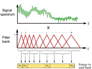
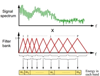
Filter Banks (FBanks) (dimension: 23):
$$ E_m = \sum_{k=0}^{K-1} |S(k)|^2 H_m(k), \quad m = 1, 2, \ldots, 23 $$
where $H_m(k)$ is the $m$-th mel filter’s frequency response, and the mel scale is:
$$ \text{mel}(f) = 2595 \log_{10}\left(1 + \frac{f}{700}\right) $$
Mel-scale filter bank energies
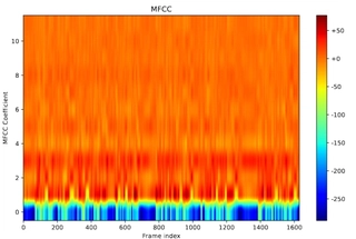
Mel-Frequency Cepstral Coefficients (MFCCs) (dimension: 12):
Cepstral coefficients from mel filter banks:
$$ c_n = \sum_{m=1}^{M} \log E_m \cos\left( n \left(m - 0.5\right) \frac{\pi}{M} \right), \quad n = 1, 2, \ldots, 12 $$
where $E_m = \sum_{k=0}^{K-1} |S(k)|^2 H_m(k)$ is the $m$-th filter bank energy, and $M = 23$.
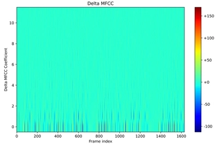
Delta MFCCs (dimension: 12): First-order differences of MFCCs:
$$ \Delta c_n(t) = \frac{\sum_{d=1}^D d \left( c_n(t shap-d) - c_n(t-d) \right)}{2 \sum_{d=1}^D d^2}, \quad n = 1, 2, \ldots, 12 $$
where $c_n(t)$ is the $n$-th MFCC at frame $t$, and $D$ is the window size (typically 2–3).
Delta-Delta MFCCs (dimension: 12):
Second-order differences:
$$ \Delta^2 c_n(t) = \frac{\sum_{d=1}^D d \left( \Delta c_n(t+d) - \Delta c_n(t-d) \right)}{2 \sum_{d=1}^D d^2}, \quad n = 1, 2, \ldots, 12 $$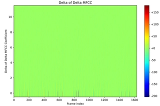

5. Classification Models

models I trained trained:

Deep Neural Network (DNN):
- Architecture: Input (69) → 64 (ReLU, Dropout 0.5) → 32 (ReLU, Dropout 0.5) → 16 (ReLU, Dropout 0.5) → 1 (Sigmoid).
- Loss: Binary Cross-Entropy.
- Training: 10 epochs, Adam optimizer.
Logistic Regression
- Use sklearn()
Linear Support Vector Machine (SVM):
- Use sklearn()
Gaussian Mixture Model (GMM):
- Construct by myself
- Models classes as Gaussian mixtures
- Trained with Expectation-Maximization.
- Its performance is not so good, I will spare some time to figure it out.

6. Experimental Results

Models were tested with frame lengths (320–4096) and shifts (80–2048). DNN outperformed others (frame length 4096, shift 1024):

Model	AUC	EER	Accuracy	Precision	Recall	F1 Score
DNN	0.9876	0.0464	0.9603	0.9765	0.9749	0.9757
Logistic Regression	0.9457	0.1134	0.9432	0.9347	0.9389	0.9368
Linear SVM	0.8937	0.9413	0.1170	0.9349	0.9352	0.9350

7. Visualization on time domain division

I restored the framed labels back to the time domain and visualized them as follows: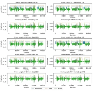

Usage

Clone the repository:

git clone https://github.com/xuankunyang/Voice-Activity-Detection.git

Install dependencies:
```
pip install -r requirements.txt
```
Extract the features first and train a binary classifier, predict, time-domain restoration, visulize the time division. Considering the space limit, I couldn’t put my pre-trained models here, but its not difficult to implement all above using this framework.
Explore visualizations in vad/latex/figs/ and the report.

Contributing

Fork the repository, create a branch, and submit pull requests. For major changes, open an issue.

🎙️ Voice Activity Detection